You know scatterplots—those sprinkles of points that help you get an initial sense for how two variables relate to one another. If you have data to analyze, you’ll probably be making a scatterplot sooner or later. In this post, I’ll run through seven ways to make scatterplots using a variety of tools in Excel, Python, and R. I’ll always use the same data, so you can easily compare and decide what works for you.
The data
The data I’m using is well known to students of data science: it’s the diamonds dataset that comes with ggplot2, a data visualization library for R (and also used in Python). You can download a copy from GitHub or access it directly when using ggplot2. Here’s the rundown:
- It contains got over 53,000 rows and 10 columns.
- Each row represents a diamond.
- The columns represent features of those diamonds: cut, color, clarity, carat weight, price, and dimensions.
Today I’m interested in the relationship between carat weight and price. I want to get a general sense of how these variables are related, so I’m going to plot carat weight on the x-axis and price on the y-axis. From time to time I’ll add in another variable—cut—as a color code applied to the points.
I’m not doing any cleaning or preprocessing of the data, just diving in for a quick look. Let’s go!
#1. Excel
Good ol’ Microsoft Excel and I have had a lot of quality time together in the last decade. I used it a bunch while analyzing data as part of my dissertation research. I used it in my last job to wrangle museum and library collections metadata. Let’s see what my old pal can do with 53,000 diamonds.
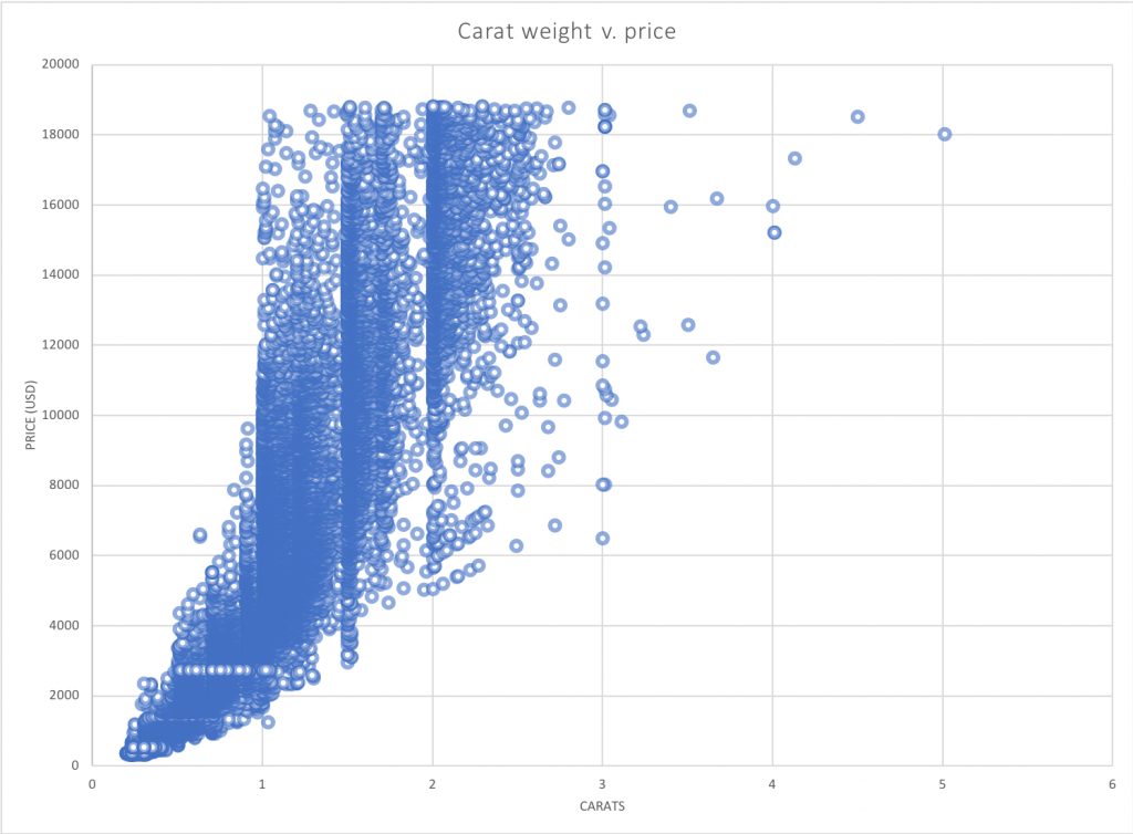
Not bad for a start! I selected this style from among the templates because the points were a little transparent, which can help us see where they pile up. The version of Excel I’m using has a convenient button to let me add elements like axis titles piecemeal, which is kind of nice. I thought about plotting the data again with a color code for cut, but it’s not easy to add an aesthetic element like that to a plot if your data isn’t already structured in a particular way. Instead, I decided to move on and see what I could do in Python.
#2. Matplotlib
I have to admit, I am frequently frustrated with Matplotlib, the biggest basic data visualization package for Python. Yes, there are a million options. Yes, with enough time and patience I could figure out how to make my plot look any way I want. But patience and time are in short supply, and with Matplotlib it feels like I never quite get what I want on the first try.
For those of you interested in the code, here’s the setup:
# Import needed packages and data
import pandas as pd
import matplotlib.pyplot as plt

diamonds = pd.read_csv('diamonds.csv')

# Create a basic scatter plot using Matplotlib
plt.figure(figsize=(12,8))
plt.scatter(diamonds['carat'], diamonds['price'], alpha=0.4)
plt.title('Carat weight v. price of diamonds', fontsize=18)
plt.xlabel('Carats')
plt.ylabel('Price (USD)')
plt.show()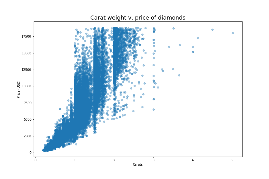
Not bad for a plot with minimal customization! I made the title a little bigger than the default size and added x- and y-axis labels. I also made the points semi-transparent so we can better see where they overlap. The plain white background, the black lines and lettering, and the font are all defaults, but Matplotlib has other styles one can choose. I think this is a little more modern and clean-looking than the one from Excel.
What if we added a little more color?
#3. Matplotlib plus color
In this next plot I wanted to color-code the points according to their cut (Fair, Good, Very Good, Premium, and Ideal) to see if there are any interesting patterns. Unfortunately, this was a little more challenging than I had hoped. I specifically wanted colors that would be legible to folks with various forms of colorblindness. This is easier to do in Seaborn, for instance, where there’s a pre-fab palette suitable for colorblindness. Today I ended up making my own by copying the hex codes for the IBM palette from davidmathlogic.com. Then I had to add a column to my data to specify what color each cut should be.
# Map colors to the unique values of the 'cut' column
colors = ['#648FFF','#785EF0','#DC267F','#FE6100','#FFB000']
categories = np.unique(diamonds['cut'])
color_dict = dict(zip(categories, colors))
diamonds['cut_category'] = diamonds['cut'].apply(lambda x: color_dict[x])

# Create a plot that colors points by values in the 'cut' column
fig, ax = plt.subplots(figsize=(12,8))
for cut in diamonds['cut'].unique():
    data = diamonds[diamonds['cut'] == cut]
    ax.scatter(data['carat'], data['price'],
               c=data['cut_category'], label=cut, alpha=0.3)
ax.legend()
plt.title('Carat weight v. price of diamonds', fontsize=18)
plt.xlabel('Carats')
plt.ylabel('Price (USD)')
plt.show()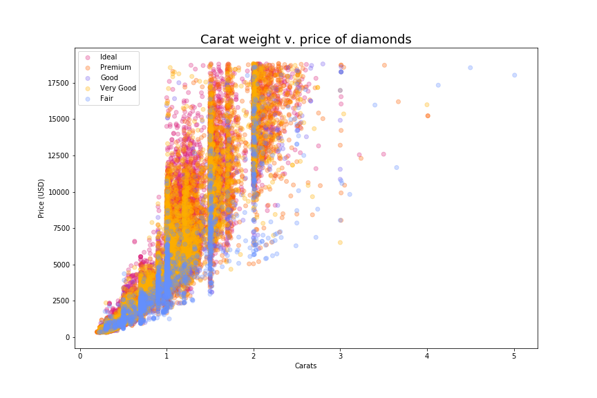
Handy! My cuts are out of rank order (oops), but at least I can see that “Fair” diamonds occur at all sizes and price points, even the really high ones, while the “Ideal” diamonds tend to be smaller in size and spread across the range of prices.
You know who would be great at making an elegant, colorful plot like this? Seaborn! Let’s try that next.
#4. Seaborn
Seaborn is a data visualization package for Python, and it is built on Matplotlib, so it’s easy to combine the two when building and customizing a plot. The magic of Seaborn, however, is that you can build beautiful things with very little code.
# Import seaborn
import seaborn as sns

# Plot the same data using seaborn
plt.figure(figsize=(14,8))
sns.scatterplot(diamonds.carat, diamonds.price,
                hue=diamonds.cut, style=diamonds.cut,
                palette='colorblind', alpha=0.3)
plt.title('Carat weight v. price of diamonds', fontsize=18)
plt.xlabel('Carats')
plt.ylabel('Price (USD)')
plt.legend()
plt.show()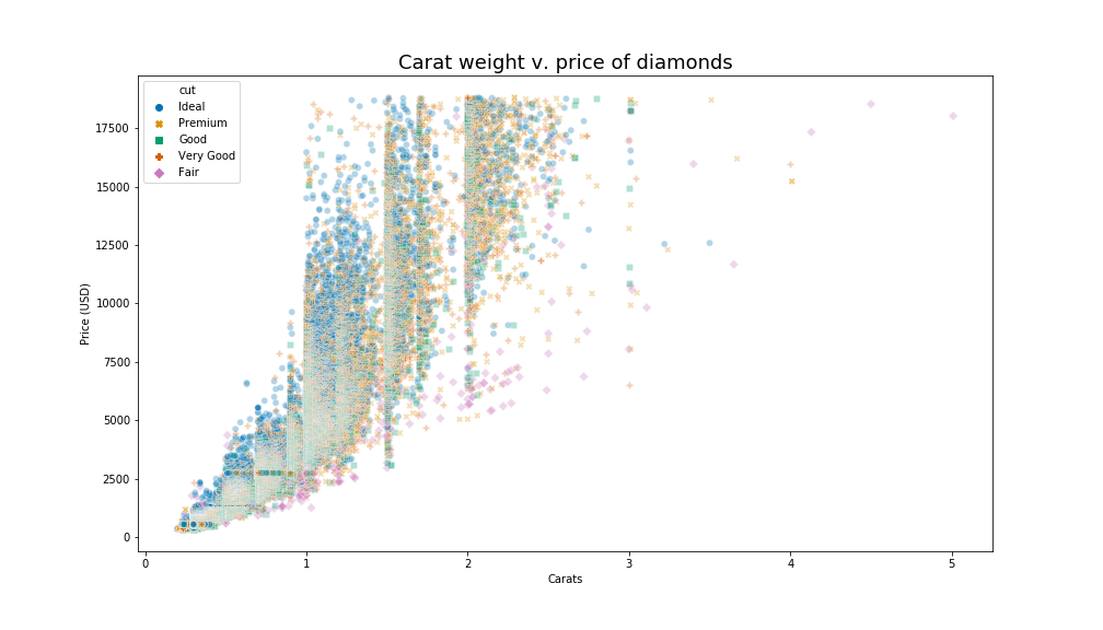
To make a similar plot in base Matplotlib, I built my own colormap and then used a for loop to assign each cut to a color and add those points to the plot. (There’s probably an easier way, but I’m a newbie data scientist, and that’s what I came up with. Thanks, Stack Overflow!) Here in Seaborn, I simply told the magical plotting machine to color the points according to the values in the ‘cut’ column of the dataset. I used a colorblind-friendly palette, which is available by default in Seaborn. With three extra words, I made the points different shapes according to cut, which helps distinguish them even more.
Now I’m looking at three features of the data at once…but what if I want more? Seaborn offers a handy way to do a lot of exploratory visualization in one fell swoop. Read on to learn about the fabulous pairplot.
#5. Seaborn pairplot
Behold:
sns.pairplot(diamonds)
plt.show()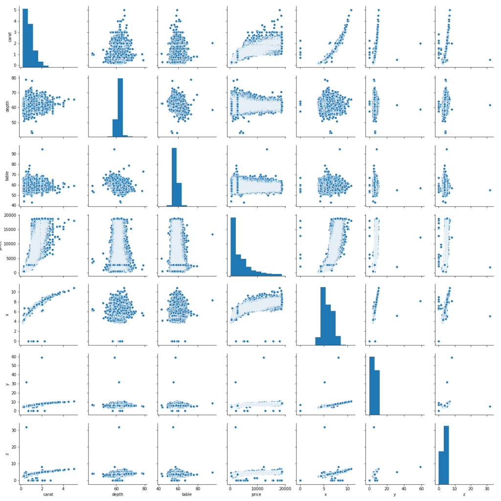
Ain’t it grand? The pairplot shows us every numerical variable pitted against every other numerical variable. On the diagonal are histograms for each variable. Now, you wouldn’t want to do a pairplot if you have dozens (or hundreds) of columns in your dataset, but at this scale, we get a glimpse of some potential relationships in our data that might help us ask better, more focused questions.
Best of all: look at that code! So brief, yet so powerful. Call me spoiled, but this is what I want when I’m exploring some data: a few short lines, then bang! Something that sparks a bunch of questions.
Speaking of spoiled, have you even tried ggplot2? Read on for a look at my personal favorite visualization library (so far).
#6. ggplot2
ggplot2 is a data visualization library for R, and the way that we construct a plot in ggplot2 just feels logical to me. First we initialize a plot by telling ggplot() which parts of our data to use. Then we add stuff to the plot’s base layer: points, a title, and x- and y-axis labels. Take a look:
# Load the tidyverse package and data
library(tidyverse)
data(diamonds)

# Create the plot
ggplot(diamonds, aes(carat, price, color=cut, alpha=0.3)) +
  geom_point() +
  ggtitle('Carat weight v. price') +
  xlab('carats') +
  ylab('price (USD)')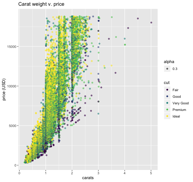
Looks good straight out the gate. Note that the levels in the color scale (based on values in the “cut” column) are in the correct order from “Fair” to “Ideal,” and I didn’t have to tell ggplot() to make that legend (it just did). The color palette being used here is viridis, which works for users with some types of colorblindness. I didn’t have to specify that, either. Once you get the basic “grammar” of ggplot2, it takes no more time to build a plot than to decide which parts of your data you want to visualize.
For my last trick, I’ll show you how to add a trend line to a scatterplot in ggplot2. Read on.
#7. ggplot2 with smoothing
According to the documentation for geom_smooth(), it “aids the eye in seeing patterns in the presence of overplotting.” We’ve got loads of overplotting in our graph, so much so that it’s hard to tell what’s going on with the diamonds under two carats and $10,000. Let’s see what geom_smooth() can do for us.
ggplot(diamonds, aes(carat, price, color=cut, alpha=0.3)) +
  geom_point() +
  geom_smooth() +
  ggtitle('Carat weight v. price') +
  xlab('carats') +
  ylab('price (USD)')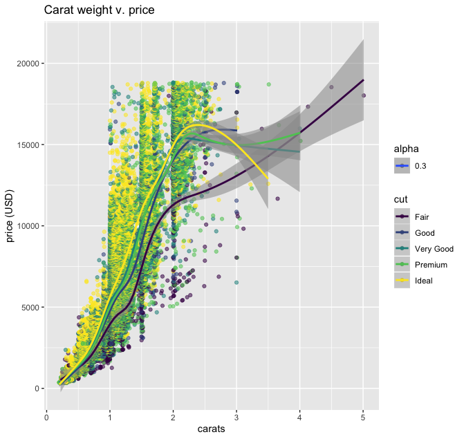
Now we see a line estimating the mean of our data as carat weight increases for each of our cut types. This definitely makes it easier get some insights from the heavily overplotted data. For instance, at the $5,000 price point, “Fair”-cut diamonds are on average about a quarter-carat bigger than all the other cuts, which are bunched up around the one-carat mark. One little addition to our code got us this insight, which we might not have been looking for otherwise.
There you have it: seven ways to scatterplot. I hope you find one that works for you.