For my first project as a Flatiron School data science bootcamper, I was asked to analyze data about the sale prices of houses in King County, Washington, in 2014 and 2015. The dataset is well known to students of data science because it lends itself to linear regression modeling. You can take a look at the data over at Kaggle.com.
In this post, I’ll describe my process of cleaning this dataset to prepare for modeling it using multiple linear regression, which allows me to consider the impact of multiple factors on a home’s sale price at the same time.
Defining my dataset
One of the interesting things about this dataset is that King County is home to some pretty massive wealth disparity, both internally and in comparison with state and national averages. Some of the world’s richest people live there, and yet 10% of the county’s residents live in poverty. Seattle is in King County, and the median household income of $89,675, 49% higher than the national average, can probably be attributed in part to the strong presence of the tech industry in the area. Home prices in the dataset range from a modest $78,000 to over $7 million.
# Import needed packages
import pandas as pd
import numpy as np
import matplotlib.pyplot as plt
import seaborn as sns

# Read in the data and view summary statistics
data = pd.read_csv('kc_house_data.csv')
data.describe()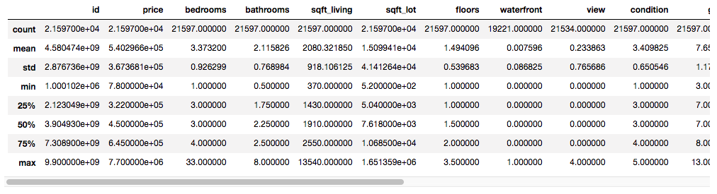
These disparities mean that it is hard to find a linear model that can describe the data while keeping error reasonably low. Common sense tells us that a twelve-bedroom house isn’t simply four times bigger than a three-bedroom house; it’s a mansion, a luxury villa, a thing of a different nature than a typical family home.
While exploring this dataset, I decided that not only was I unlikely to find a model that could describe modest homes and mansions alike, I also didn’t want to. Billionaires, if you’re reading this: I’m sure there is someone else who can help you figure out how to maximize the sale price of your Medina mansion. I would rather use my skills to help middle-income families understand how they can use homeownership to build wealth.
This thinking brought me to my first big decision about cleaning the data: I decided to cut it down to help me focus on midrange family homes. I removed the top 10% most expensive homes and then limited the remaining data to just those homes with 2 to 5 bedrooms.
# Filter the dataset
midrange_homes = data[(data['price'] < np.quantile(data['price'], 0.9))
                         & (data['bedrooms'].isin(range(2, 6)))]

# View summary statistics
midrange_homes.describe()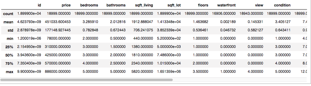
All told, this left me with 18,999 homes with a median sale price of $425,000. A little fiddling with a mortgage calculator persuaded me that this could be an affordable price for a family making the median income of $89,675, assuming they had excellent credit, could make a 14% downpayment, and got a reasonable interest rate.
Limiting the price and number of bedrooms had a nice collateral effect of making most of the extreme values in the dataset disappear. At this point, I was ready to move on my first real cleaning steps: resolving missing values.
Missing no more
Many datasets come with missing values, where someone forgot or chose not to collect or record a value for a particular variable in a particular observation. Missing values are a problem because they can interfere with several forms of analysis. They may be a different data type than the other values (e.g., text instead of a number). If lots of values are missing for a particular variable or observation, that column or row may be effectively useless, which is a waste of all the good values that were there. It is important to resolve missing values before doing any quantitative analysis so that we can better understand what our calculations actually represent.
# Check for missing values by column
midrange_homes.isna().sum()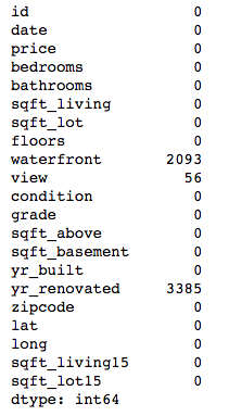
There are a couple of typical ways to resolve missing values. First, you can just remove the columns or rows with missing values from the dataset altogether. This definitely protects you from the perils of missing data, but at the expense of any perfectly good data that happened to be in one of those columns or rows.
An alternative is to change the missing values to another value that you think is reasonable in context. This could be the mean, median, or mode of the existing values. It could also be some other value that conveys “missingness” while still being accessible to analysis, like 0, ‘not recorded,’ etc.
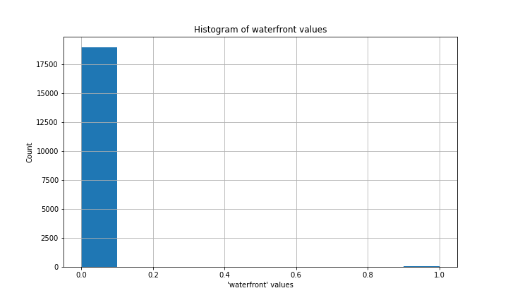
My dataset had missing values in three columns: waterfront, view, and yr_renovated.
waterfront records whether a house is on a waterfront lot, with 1 apparently meaning “yes” and 0 “no.”
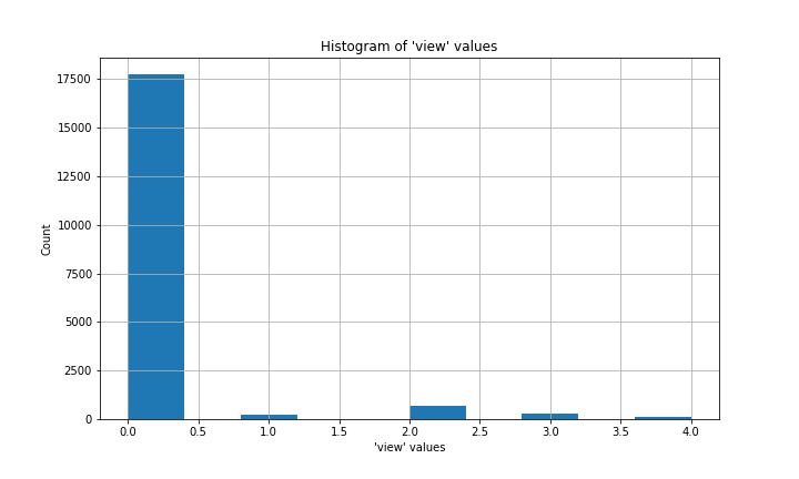
The meaning of the view column is not entirely clear. If you do some searching through other people’s uses of this dataset, you’ll see it interpreted in various ways. The best interpretation I found was that it reflects how much a house was viewed before it sold, and the numeric values (0 to 4) probably represent tiers of a scale rather than literal numbers of views.
yr_renovated is also a bit tricky. The vast majority of values are 0, with other values concentrated in the last few decades before 2014/2015.
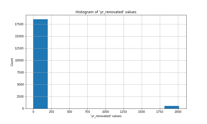
In each case, 0 was the most common value (the mode) by a long shot. I’ll never know whether the folks who recorded this data meant to put 0 for each missing value, or if those values were truly unknown. Under the circumstances, filling the missing values with 0 wouldn’t make a substantial difference to the overall distribution of values, so that is what I chose to do.
# Fill missing values with 0, the mode of each column
midrange_homes['waterfront'] = midrange_homes['waterfront'].fillna(0.0)
midrange_homes['waterfront'] = midrange_homes['waterfront'].astype('int64')

midrange_homes['view'] = midrange_homes['view'].fillna(0.0).astype('int64')

midrange_homes['yr_renovated'] = midrange_homes['yr_renovated'].fillna(0)
midrange_homes['yr_renovated'] = midrange_homes['yr_renovated'].astype('int64')
Not my type
Looking at the info on this dataset, we can see that two columns—date and sqft_basement—are “objects” (i.e., text) while the rest are numbers (integers or decimal values, a.k.a. floats). But dates and basement square footage are values that I will want to treat like numbers, so I need to changes these columns to new datatypes.
# Review column datatypes
midrange_homes.info()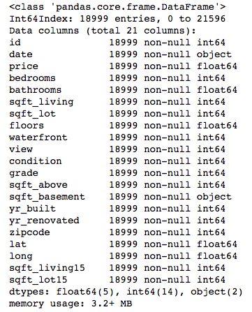
date is a little tricky because it contains three pieces of information (day, month, and year) in one string. Converting it to a “datetime” object won’t do me much good; I know from experimentation that my regression model doesn’t like datetimes as inputs. Because all the observations in this dataset come from a short period in 2014-2015, there’s not much I can learn about changes over time in home prices. The month of each sale is the only part that really interests me, because it could help me detect a seasonal pattern in sale prices.
I use the string .split() method in a list comprehension to grab just the month from each date and put it into a new column. The original date column can now be eliminated in the next step.
# Create 'month' column
midrange_homes['month'] = [x.split('/')[0] for x in midrange_homes['date']]
midrange_homes['month'] = pd.to_numeric(midrange_homes['month'],
                                        errors='coerce')
Stop, drop, and .info()
Now I’m ready to drop some columns that I don’t want to consider when I build my multiple linear regression model.
I don’t want id around because it is supposed to be a unique identifier for each sale record—a serial number, basically—and I don’t expect it to have any predictive power.
date isn’t needed anymore because I now have the month of each sale stored in the month column.
Remember sqft_basement, a numeric column trapped in a text datatype? I didn’t bother coercing it to integers or floats above because I noticed that sqft_living appears to be the sum of sqft_basement and sqft_above. My focus is on things that a family can do to maximize the sale price of their home, and I doubt many people are going to shift the balance of above- versus below-ground space in their homes without also increasing overall square footage. I’ll drop the two more specific columns in favor of using sqft_living to convey similar information.
# Drop unneeded columns
midrange_homes.drop(['id', 'date', 'sqft_above', 'sqft_basement'],
                    axis=1, inplace=True)

# Review the remaining columns
midrange_homes.info()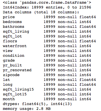
What remains is a DataFrame with 18,999 rows and 18 columns, all numeric datatypes, perfect for regression modeling.
It’s categorical, dummy
So I fit models to a few minor variations of my dataset, but the results weren’t what I wanted. I was getting adjusted R-squared values around 0.67, which meant that my model was only describing 67% of the variability in home price in this dataset. Given the limits of the data itself—no info on school districts, walkability of the neighborhood, flood risk, etc.—my model is never going to explain 100% of the variability in price. Still, 67% is lower than I would like.
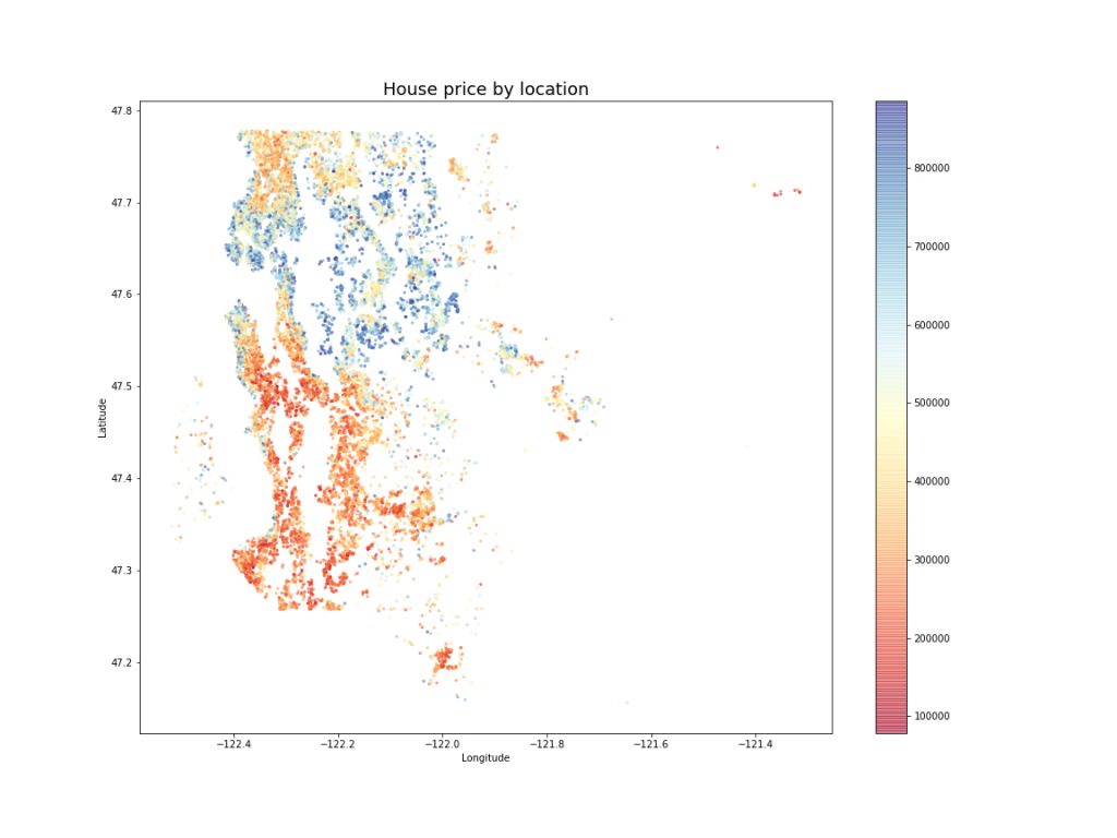
As I mentioned above, King County is home to some extremes of wealth, and even though I excluded the most expensive houses from my dataset, I didn’t exclude their more modest neighbors. The locations of the houses, expressed through zipcode, could be having an effect on price. On my instructor’s advice, I tried one-hot encoding on the zipcode column.
# Generate dummy variables
zip_dummies = pd.get_dummies(midrange_homes['zipcode'], prefix='zip')

# Drop the original 'zipcode' column
mh_no_zips = midrange_homes.drop('zipcode', axis=1)

# Concatenate the dummies to the copy of 'midrange_homes'
mh_zips_encoded = pd.concat([mh_no_zips, zip_dummies], axis=1)

# Drop one of the dummy variables
mh_zips_encoded.drop('zip_98168', axis=1, inplace=True)
One-hot encoding, also known as creating dummy variables, takes a variable and splits each unique value off into its own column filled with zeroes and ones. In this case, I ended up with a column for each zipcode in the dataset, filled with a 1 if a house was in that zip code and 0 if not. I then dropped one zipcode column arbitrarily to represent a default location. The coefficients my model generated for the other zipcodes would represent what a homeowner stood to gain or lose by having their home in those zipcodes as opposed to the dropped one.
Treating zipcodes as a categorical variable instead of a continuous, quantitative one paid off immediately: the adjusted R-squared value jumped to 0.82. My model could now explain 82% of the variability in price across this dataset. With that happy outcome, I was ready to move on to validating the model, or testing its ability to predict the prices of houses it hadn’t encountered yet.
That’s a summary of how I explored and cleaned the data for my project on house prices in King County, Washington. You can read my code or look at the slides of a non-technical presentation of my results over on my GitHub repository. You can also watch my non-technical presentation on YouTube.